Philosophy, Computing, and Artificial Intelligence

×

Deep learning is a kind of machine learning that works by training neural networks.

To begin to see what goes on in deep learning, we start by thinking about neurons.

Artificial Neurons

⊕


Perceptron

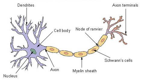
The neurons in deep learning are computational models of biological neurons.

A biological neuron has dendrites, a cell body, and an axon. The dendrites (from the Greek δενδρίτης) take input from other neurons in the form of electrical impulses. The cell body processes these impulses, and the output goes from axon terminals to other neurons.

According to an estimate in 2009, the average male human brain has 86 billion neurons.

Perceptron Neurons

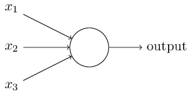
A perceptron is an example of an artificial neuron.

It takes a series of 0's and 1's as inputs (x₁ ... x_m) and computes a 0 or 1 as output.

The computation is a function of weights (w₁ ... w_m) and a threshold value. If the sum w₁x₁ + ... + w_mx_m is greater than the threshold value, the output is 1. Otherwise, it is 0. ⊕


Perceptrons can implement truth-functions. Conjunction (φ ∧ ψ) is an example. Let the perceptron have two inputs, each with a weight of 0.6, and a threshold value of 1. If both inputs are 1, the sum exceeds the threshold value of the perceptron and thus the output is 1. Otherwise, the output is 0. With these conditions for activating the perceptron, the output matches the truth-table for conjunction.

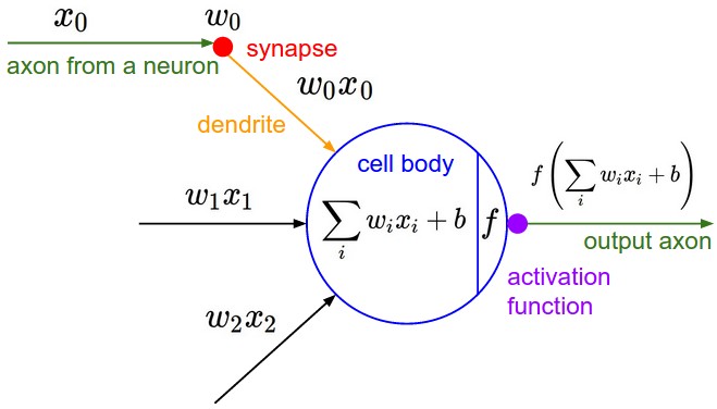
A perceptron is an instance of the integrate-and-fire model.

A neuron receives inputs through synapses. The weights represent the efficiency with which a synapse communicates inputs to the cell body. This means that some inputs to weigh more heavily than others in the computation. The neuron is quiet unless the threshold is crossed.

The computation in a perceptron is typically expressed mathematically as a dot product of a vector of weights and a vector of inputs. The negative of the threshold value is the perceptron's bias, b. The value of the dot product is 1 if w · x + b > 0 and 0 otherwise.

Sigmoid Neurons

⊕





"Suppose we arrange for some automatic means of testing the effectiveness of any current weight [and bias] assignment [in the neuron] in terms of actual performance and provide a mechanism for altering the weight [and bias] assignment so as to maximize the performance. We need not go into the details of such a procedure to see that it could be made entirely automatic and to see that a machine so programed would 'learn' from its experience" (Arthur L. Samuel, "Artificial Intelligence: A Frontier of Automation," 17. The Annals of the American Academy of Political and Social Science. Vol. 340, Automation, 10-20, 1962).



A sigmoid neuron has an important feature a perceptron lacks: small changes in the weights and bias cause small changes in the output. This allows sigmoid neurons to "learn."

We can make a neuron "learn" by changing its weights and biases. We know what the output should be. If it does not output this value, we change the weights and biases so that the output is closer to what it should be. In this way, the neuron "learns" what its output should be.

This talk about the neuron "learning" trades on the pretense that the neuron itself is changing its weights and biases in an effort to correct its mistakes. When it sees that its output is not what it should be, it adjusts its weights and biases in an effort to do better. Through many iterations of "learning," the neuron's output approaches the correct output. The neuron, in this way, "learns" like an archer who, after each shot, tries to get closer to hitting the target by slightly adjusting the angle of the arrow and how far he pulls back the string.

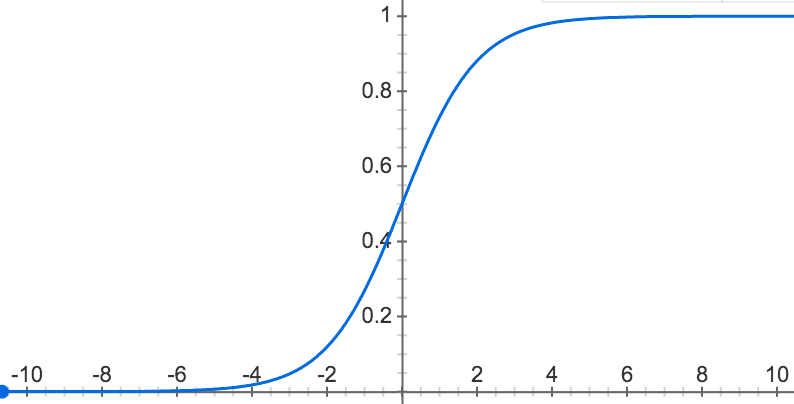
A sigmoid neuron has the parts we see in a perceptron (inputs, weights, a bias, and an output), but the inputs and outputs in a sigmoid neuron may have any value from 0 to 1. The activation function is also different. In a sigmoid neuron, it is the sigmoid function.

The Sigmoid Function

The sigmoid function is σ(x) = ` 1/(1 + e^-x)`, where x = w · x + b

This function (which is scary looking) is a technical device. It maps w · x + b to a smooth curve that preserves desirable features of the activation function for perceptrons.

We can see this if we note the following two facts. When w · x + b is a large positive number, the value of the sigmoid function is close to 1 because `e^-x` is close to 0. When w · x + b is a large negative number, the function is close to 0 because `e^-x` is extremely large.

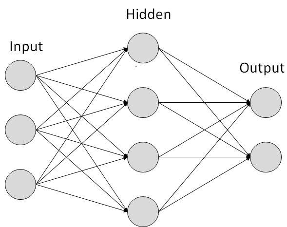
Artificial Neural Networks

⊕ Artificial neurons may be linked together in a feedfoward neural network in which the output from one layer is input for the next layer. The first layer is the input layer. The last layer is the output layer. The hidden layers are the neurons that are neither the input nor output layers.

A feedforward network of artificial neurons may be understood as a device that makes "decisions about decisions." The first layer of neurons makes a "decision" about the input, the next layer makes a "decision about the decision" of the prior layer, and so on.

We are going to consider a feedforward neural network that classifies handwritten digits.

This neural network is the "Hello World" in the field of deep learning.

(This way of talking comes the practice of introducing programming languages to students by making them write a program that prints "Hello, World!" This practice started in the 1970's.)

A Feedforward Network to Classify Digits

⊕ For a good video (YouTube) introduction to MNIST, see the series Neural Networks, by 3Blue1Brown.




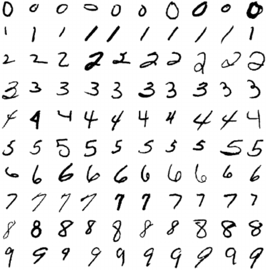
In grayscale, the intensity of light for each pixel is represented as a number from 0 to 255. 0 represents "black" (no light), 255 represents "white" (all light), and values in between 0 and 255 represent decreasing shades of "gray". The MNIST dataset was assembled in the 1980's. It contains images of handwritten digits.

MNIST is a (M) modified subset of two datasets (Special Database 1 and Special Database 3) of images of handwritten digits that the National Institute of Standards and Technology (NIST) collected. Special Database 1 was collected from high school students. Special Database 3 was collected from employees of the US Census Bureau. The MNIST data selects from both of the two datasets and normalizes the images so that each is 28 x 28 pixels in greyscale.

The images in the dataset are split into 60,000 training images and 10,000 test images.

The input to each neuron in the input layer in the network is one pixel from the input image. Since each image is 28 x 28 pixels, the input layer has 784 (or 28 x 28) neurons.

The input layer is part of a neural network of sigmoid neurons. Because the 28 x 28 images in the MNIST dataset are in greyscale, each is represented as a NumPy (the package for scientific computing with Python) one-dimensional array of 784 values between 0 and 1.

The output layer in the network has 10 neurons. The first neuron in this layer indicates whether the image is a 0, the second whether it is a 1, the third whether it is a 2, and so on.

Minimizing the Error Function

⊕

This network needs to "learn," or be "trained," to classify the digits correctly.

The amount of error in a network is sensitive to its weights and biases. Training or learning in a network is a matter of finding a set of weights and biases that minimize the error.

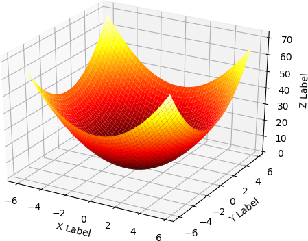
This is where things begin to get a little difficult, but we can begin to get some insight into how this minimization works. We consider the relatively simple function `f(x,y) = x^2 + y^2` and how we might move in small steps to values that minimize the value of this function.

`gradf(x,y)` is the gradient of `f(x,y)`. The gradient is a function. It takes two coordinates as a point in the space and returns two coordinates in the direction of steepest ascent.

`gradf(x,y) = [[(delf)/(delx)(x,y)], [(delf)/(dely)(x,y)]] = [[2x],[2y]] `.

If the starting-point is `(1,3)` for the ascent, the direction of steepest ascent is toward

`[[2*1],[2*3]] = [[2],[6]] `

We want to move in the direction of steepest descent, so we take negative steps.

Let the step size be `eta = 0.01`. If we step from `(1,3)` to `(2,6)`, we reach `(0.98,2.94)`. In the `x` direction, we step to `-0.01*2`. In the `y` direction, we step to `-0.01*6`.

The value of `f(x,y)` at `(1,3)` is `10`. The value at `(0.98,2.94)` is `9.604`.

From the new position, the steepest ascent is toward

`[[2*0.98],[2*2.94]] = [[1.96],[5.88]] `

Stepping again takes us to `(0.9604,2.8812)`. Here the value of `f(x,y)` is `9.2236816.`

With each step from `(1,3)`, the value of the function `f(x,y) = x^2 + y^2` decreases.

An Example Image from the MNIST Data Set

Now lets take a look at an image we want our neural network to classify correctly.

The image below of the digit 5 is an image in training_data.

training_data is a list of 60,000 2-tuples (x, y).
x is a 1-D array of 784 pixel intensities that represents image.
y is a 1-D array of 10 of elements that functions as the label for image.

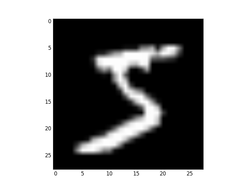
training_data[0] is the first tuple.
training_data[0][0] is the x in the first tuple.
training_data[0][1] is the y in the first tuple. ⊕ I use the source code ((c) 2012-2018 Michael Nielsen) from Michael Nielsen's Neural Networks and Deep Learning. He has made it available in a GitHub repository.

To get a copy of this source code, I installed Git onto my Linux distribution (Arch Linux), made a directory I named "git," changed the current directory to the one I made, and created a copy (or "clone") of the repository:

% sudo pacman -S git
% mkdir git
% cd git
% git clone https://github.com/mnielsen/neural-networks-and-deep-learning.git

Nielsen's Python code is in Python 2.6 or 2.7. Michal Daniel Dobrzanski has a repository with code in Python 3.5.2.

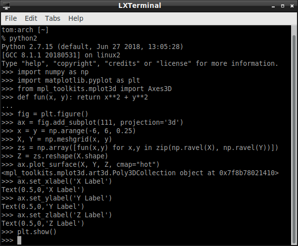
tom:arch [~/git/neural-networks-and-deep-learning/src]
% python2
Python 2.7.12 (default, Jun 28 2016, 08:31:05)
[GCC 6.1.1 20160602] on linux2
Type "help", "copyright", "credits" or "license" for more information.
>>> import mnist_loader

>>> training_data, validation_data, test_data = mnist_loader.load_data_wrapper()
>>> training_data[0][1].shape
(10, 1)
>>> training_data[0][1]
array([[ 0.],
       [ 0.],
       [ 0.],
       [ 0.],
       [ 0.],
       [ 1.], # the image shows a "5"
       [ 0.],
       [ 0.],
       [ 0.],
       [ 0.]])
>>> training_data[0][0].shape
(784, 1)
>>> import numpy as np
>>> image_array = np.reshape(training_data[0][0], (28, 28))
>>> import matplotlib.pyplot as plt
>>> image = plt.imshow(image_array, cmap ='gray')
>>> plt.show()	

Making the MNIST Dataset Ready

mnist.pkl.gz is a "pickled" tuple of 3 lists: the training set (training_data), the validation set (validation_data), and the testing set (test_data).

(The talk of "pickling" is in analogy to food. Pickling is a process that preserves food for later use. Python provides gives users a way to "pickle" objects to preserve them for later use.)

The function load_data_wrapper() returns training_data, validation_data, test_data.

validation_data and test_data are lists containing 10,000 2-tuples (x, y).
x is a 1-D array of 784 pixel intensities that represents the image.
y is a 1-D array of 10 elements that function as the label for image.

We are not going to use the validation_data.

import cPickle 
import gzip
import numpy as np

def load_data():
    f = gzip.open('../data/mnist.pkl.gz', 'rb')
    training_data, validation_data, test_data = cPickle.load(f)
    f.close()
    return (training_data, validation_data, test_data)

def load_data_wrapper():
    tr_d, va_d, te_d = load_data()
    training_inputs = [np.reshape(x, (784, 1)) for x in tr_d[0]]
    training_results = [vectorized_result(y) for y in tr_d[1]]
    training_data = zip(training_inputs, training_results)
    validation_inputs = [np.reshape(x, (784, 1)) for x in va_d[0]]
    validation_data = zip(validation_inputs, va_d[1])
    test_inputs = [np.reshape(x, (784, 1)) for x in te_d[0]]
    test_data = zip(test_inputs, te_d[1])
    return (training_data, validation_data, test_data)

def vectorized_result(j):
    e = np.zeros((10, 1))
    e[j] = 1.0
    return e

The Rest of the Python Program

We will not try to understand in the source code (which belongs (Copyright (c) 2012-2018 Michael Nielsen) to Michael Nielsen) or the underlying algorithm in complete detail.

The Network Class

class Network(object):

    def __init__(self, sizes):
        self.num_layers = len(sizes)
        self.sizes = sizes
        self.biases = [np.random.randn(y, 1) for y in sizes[1:]]
        self.weights = [np.random.randn(y, x) for x, y in zip(sizes[:-1], sizes[1:])]

In the program, we use this class to create a 784x20x10 neural network (784 neurons in the input layer, 30 in the hidden layer, and 10 in the output layer).

sizes = [784,30,10], sizes[1:] = [30,10], sizes[:-1] = [784,30]

An Example Network

The following code creates a neural network (net) whose input layer has two neurons, whose middle layer has three neurons, and whose output layer has one neuron.

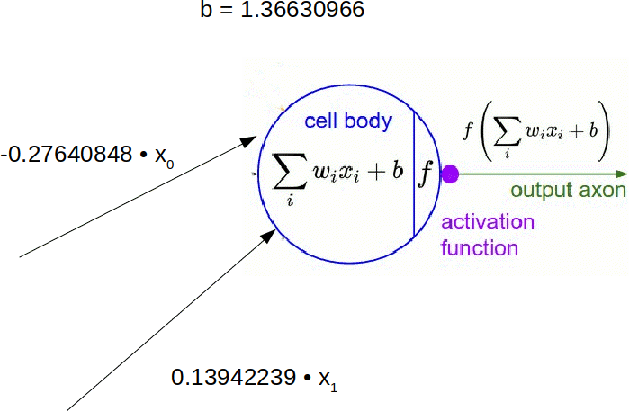
The biases and weights are set as random numbers. The input layer has no bias. Biases are only used in computing the output from later layers.

For the [2, 3, 1] network, the biases are in a 3 x 1 array and a 1 x 1 array.

tom:arch [~/git/neural-networks-and-deep-learning/src]
% python2
Python 2.7.12 (default, Jun 28 2016, 08:31:05)
[GCC 6.1.1 20160602] on linux2
Type "help", "copyright", "credits" or "license" for more information.
>>> import network
>>> net = network.Network([2, 3, 1])
>>> net.biases[0].shape
(3, 1)
>>> net.biases[0]
array([[ 1.36630966],
       [ 1.05788544],
       [ 0.80606255]])
>>>net.biases[1].shape
(1, 1)
>>>net.biases[1]
array([[ 1.54813682]])
>>>	

⊕





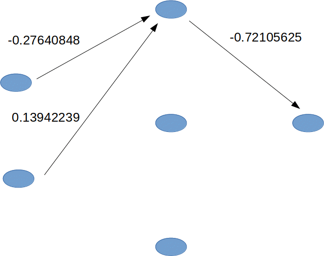
For the [2, 3, 1] network, the weights are in a 3 x 2 array and a 1 x 3 array.

The first row in net.weights[0] are the weights the first neuron in the hidden layer attributes to the outputs of the first and second neurons in the input layer.

>>> net.weights[0].shape
(3, 2)
>>> net.weights[0]
array([[-0.27640848,  0.13942239],
       [ 1.13350606,  1.51767629],
       [-0.03836741,  0.06409297]])
>>> net.weights[1].shape
(1, 3)
>>> net.weights[1]
array([[-0.72105625,  1.76366748,  1.49408987]])
>>> 

Stochastic (Mini-Batch) Gradient Descent

This is where we train the network to make it "learn" to recognize the digits.

An "epoch" in deep learning is a full pass through the training data.

For each epoch, the training data is randomly shuffled and partitioned into "mini-batches."

Once the last mini-batch is processed, the network is evaluated against the test data.

def SGD(self, training_data, epochs, mini_batch_size, eta,
        test_data=None):
    if test_data: n_test = len(test_data)
    n = len(training_data)
    for j in xrange(epochs):
        random.shuffle(training_data)
        mini_batches = [training_data[k:k+mini_batch_size] for k in xrange(0, n, mini_batch_size)]
        for mini_batch in mini_batches:
            self.update_mini_batch(mini_batch, eta)
        if test_data
            print "Epoch {0}: {1} / {2}".format(j, self.evaluate(test_data), n_test)
        else:
            print "Epoch {0} complete".format(j)	

The method update_mini_batch updates the weights and biases.

⊕ The minibatch is random sample. If the sample size is large enough, the weights and biases learned from the minibatch approximate the weights and biases that would be learned from training with all the images in the training data. For each tuple in the mini-batch, the method calculates and saves an adjustment to the weights and biases that reduces the value of the error function for the network.

The adjustment is computed by evaluating the gradient of the error function for the network at the current weights and biases in the network. This gives us the amounts we should increase or decrease the weights and biases to reduce the value of the error function.

These adjustments are accumulated across the whole mini-batch, and we take the average of these adjustments (scaled by the step size) to update the weights and biases in the network.

	def update_mini_batch(self, mini_batch, eta):
        nabla_b = [np.zeros(b.shape) for b in self.biases]
        nabla_w = [np.zeros(w.shape) for w in self.weights]
        #
        #
        #
        for x, y in mini_batch:
            delta_nabla_b, delta_nabla_w = self.backprop(x, y)
            nabla_b = [nb+dnb for nb, dnb in zip(nabla_b, delta_nabla_b)]
            nabla_w = [nw+dnw for nw, dnw in zip(nabla_w, delta_nabla_w)]
        #
        # update weights and biases
        #
        self.weights = [w-(eta/len(mini_batch))*nw for w, nw in zip(self.weights, nabla_w)]
        self.biases = [b-(eta/len(mini_batch))*nb for b, nb in zip(self.biases, nabla_b)]	

The update_mini_batch uses the method backprop to compute the adjustments.

The backprop method has two parts.

In the "feedforward" section of the method, backprop forward feeds the training input (x) through the network and stores the zs and activations layer by layer.

The zs are the input to the activation function.

The activations are the outputs of the activation function.

In the "backward pass" section, backprop uses the zs and activations to calculate the adjustments. This calculation is the most important (and difficult) part of the algorithm.

def backprop(self, x, y):
    #
    # x is the input to the network, y is the label for x
    #
    nabla_b = [np.zeros(b.shape) for b in self.biases]
    nabla_w = [np.zeros(w.shape) for w in self.weights]
    #
    # feedforward
    #
    # feed x forward through the network
    # The first time through the loop the activation is the input to the network
    #
    activation = x
    activations = [x]                                                            # list of activations layer by layer
    zs = []
    for b, w in zip(self.biases, self.weights):
        z = np.dot(w, activation)+b                                              # np.dot is the numpy dot product
        zs.append(z)
        activation = sigmoid(z)
        activations.append(activation)
    #
    #
    # backward pass
    #
    # fundamental equation 1
    # Error in the neurons in the output layer
    delta = self.cost_derivative(activations[-1], y) * sigmoid_prime(zs[-1])     # [-1] the last layer
                                                                                 # * is the Hadamard product, ⊙
    # fundamental equation 3
    # Error in biases in the neurons in the output layer
    nabla_b[-1] = delta
    #
    # fundamental equation 4
    # Error in weights in the neurons in the output layer
    nabla_w[-1] = np.dot(delta, activations[-2].transpose())
    #
    # Errors in the previous layers
    for l in xrange(2, self.num_layers):
        z = zs[-l]
        sp = sigmoid_prime(z)
        delta = np.dot(self.weights[-l+1].transpose(), delta) * sp               # fundamental equation 2
        nabla_b[-l] = delta                                                      # fundamental equation 3
        nabla_w[-l] = np.dot(delta, activations[-l-1].transpose())               # fundamental equation 4
    #
    #
    # return the errors in the weights and biases
    #
    return (nabla_b, nabla_w)


def cost_derivative(self, output_activations, y):
    return (output_activations-y) 
    
def sigmoid(z):
    """The sigmoid function."""
    return 1.0/(1.0+np.exp(-z))

def sigmoid_prime(z):
    """Derivative of the sigmoid function."""
    return sigmoid(z)*(1-sigmoid(z))

The Error Function

When an image `x` from the training set of `n` images is fed through the network, it produces a vector of outputs, `a^L`, different in general from the desired vector of outputs `y`.

We try to minimize this difference by minimizing the average error in the network

`E = 1/n ∑_x^n E_x`

where

`E_x = 1/2 norm(y - a^L)^2 = 1/2 ∑_j (y_j - a_j^L)^2` ⊕ `y_j` is the desired activation of the `j^(th)` neuron in the output layer when image `x` is the input to the network

`a_j^L`is the activation of `j^(th)` neuron in the output layer when image `x` is the input to the network

Q: Why the constant `1/2`?
A: To cancel the exponent when differentiating. We can think of it as part of the step parameter, which we set.

In the 784x30x10 neural network (the network trained (in the example below) to classify the MNIST images), there are 23,820 weights (784x30 + 30x10) and 40 biases (30 + 10). The activations in the vector `a^L(x)` are a function of these weights and biases.

(The 784x30x10 network is small. OpenAI's GPT-3 from 2020 has 175 billion parameters.)

The `L^2` (Euclidean) norm is the length of a vector from the origin to a point.

Suppose, as an example, the point is

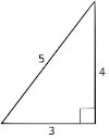⊕ `u = [[x],[y]] = [[3],[4]] `

The `L^2` norm of ` u = norm u = \sqrt{3^2 + 4^2} = 5.`

The error function uses the squared `L^2` norm to make the computation simpler. Because it eliminates the square root, the computation is sum of the squared values of the vector.

The partial derivative of `E_x` with respect to `a_j^L` is

⊕ `(delE_x)/(dela_j^L) = del/(dela_j^L)[1/2(y_j-a_j^L)^2]`

           `= 1/2 * del/(dela_j^L)[(y_j-a_j^L)^2]`

           `= 1/2 * 2(y_j-a_j^L) * del/(dela_j^L)[y_j-a_j^L]`

           `= (y_j-a_j^L) * (del/(dela_j^L)y_j - del/(dela_j^L)a_j^L) `

           ` = (y_j-a_j^L) * (0 - 1)`

            ` = (y_j-a_j^L) * -1`

           ` = a_j^L-y_j` `(delE_x)/(dela_j^L) = a_j^L-y_j`

The evaluate method returns the number of inputs for which the network output is correct.

def evaluate(self, test_data):
        # the output is the index of the first neuron in the final layer with a maximum activation
        test_results = [(np.argmax(self.feedforward(x)), y) for (x, y) in test_data]
        return sum(int(x == y) for (x, y) in test_results)

def feedforward(self, a):
    for b, w in zip(self.biases, self.weights):
        a = sigmoid(np.dot(w, a)+b)
    return a	  

Four Fundamental Equations for Training the Network

⊕ `z_j^l` is the pre-activation. It is the input to the activation function for the `j^(th)` neuron in layer `l`.

`z_j^l` is the weighted sum of all the outputs from previous layer's neurons plus the bias in neuron `j`.

`z_j^l = ∑_k w_(jk)^l a_k^(l-1) + b_j^l`.

`w_(jk)^l` is the weight on the connection into the `j^(th)` neuron in layer `l` from the `k^(th)` neuron in layer `(l - 1)`.

(subscripts: first = target neuron, second = source neuron)

`a_k^(l-1)` is the activation of the `k^(th)` neuron in layer `(l - 1)`.

`a_k^(l-1) = sigma(z_k^(l-1))`

`sigma` = the sigmoid function = the activation function.

`b_j^l` is the bias of the `j^(th)` neuron in layer `l`.



Chain Rule:

`(delz)/(dely) (dely)/(delx) = (delz)/(delx)`, if `z = f(y) and y = g(x)` We use `delta_j^L` for `(delE_x)/(delz_j^L)` and `delta_j^l` for `(delE_x)/(delz_j^l)`,
where `L` is the output layer and `l' is a previous layer in the network.

Fundamental Equation 1. Error in neurons in the output layer

`delta_j^L` = `(delE_x)/(delz_j^L)` = `(delE_x)/(dela_j^L)sigma'(z_j^L)`.
`delta_j^L` = how much neuron `j` in the output layer is responsible for the total error.

The contribution of neuron `j` to the total error is the contribution of its output scaled by how sensitive its output is to changes in its input `z_j^L`.

Proof:

`(delE_x)/(delz_j^L) = ∑_k (delE_x)/(dela_k^L) (dela_k^L)/(delz_j^L) `, by the chain rule.

` ∑_k (delE_x)/(dela_k^L) (dela_k^L)/(delz_j^L) = (delE_x)/(dela_j^L) (dela_j^L)/(delz_j^L)`, since `(delE_x)/(dela_k^L) (dela_k^L)/(delz_j^L) = 0` if `j \ne k`.

`(delE_x)/(dela_j^L) (dela_j^L)/(delz_j^L) = (delE_x)/(dela_j^L)sigma'(z_j^L)`, since `a_j^L = sigma(z_j^L)`.

Fundamental Equation 2. Error in neurons in other layers

`delta_j^l = (delE_x)/(delz_j^l) = ∑_k w_(jk)^(l+1)delta_k^(l+1)sigma'(z_j^l)`.
`delta_j^l` = how much neuron j in layer l is responsible for the total error.

The error at neuron `j` comes from all the places its output goes: the neurons `k` in the next layer. Each of those connections is weighted by `w_(jk)^(l+1)`. These weights scale neuron `j`'s contribution. Each target neuron k has an error `delta_k^(l+1)`. Neuron `j`'s contribution to the total error is thus the weighted sum of these errors scaled by how sensitive `j`'s output is to changes in its input `z_j^l`.

Proof:

`(delE_x)/(delz_j^l) = ∑_k (delE_x)/(delz_k^(l+1)) (delz_k^(l+1))/(delz_j^l)`, by the chain rule.

`∑_k (delE_x)/(delz_k^(l+1)) (delz_k^(l+1))/(delz_j^l) = ∑_k (delz_k^(l+1))/(delz_j^l) (delE_x)/(delz_k^(l+1)) = ∑_k (delz_k^(l+1))/(delz_j^l) delta_k^(l+1)`.

`(delz_k^(l+1))/(delz_j^l) = w_(jk)^(l+1)sigma'(z_j^l)`

because

`z_k^(l+1) = ∑_m w_(mk)^(l+1)a_m^l + b_k^(l+1) = ∑_m w_(mk)^(l+1)sigma(z_m^l) + b_k^(l+1)`.

Hence, `∑_k (delz_k^(l+1))/(delz_j^l) delta_k^(l+1) = ∑_k w_(kj)^(l+1)sigma'(z_j^l) delta_k^(l+1) = ∑_k w_(kj)^(l+1) delta_k^(l+1) sigma'(z_j^l) `.

Fundamental Equation 3. Error in the bias of a neuron

`(delE_x)/(delb_j^l) = delta_j^l`.

`(delE_x)/(delb_j^l)` is how much the bias of neuron `j` in layer `l` is responsible for the total error.

A change in `b_j^l` changes `z_j^l` by the same amount. So the sensitivity of the total error to changes in `b_j^l` is the same as the sensitivity of the total error to changes in `z_j^l`. This is `delta_j^l`.

Proof:

`(delE_x)/(delb_j^l) = (delE_x)/(delz_j^l) (delz_j^l)/(delb_j^l)`, by the chain rule.

`(delE_x)/(delz_j^l) = delta_j^l`, by definition. `(delz_j^l)/(delb_j^l) = 1`, since `z_j^l = ∑_k w_(jk)^la_j^(l-1) + b_j^l`.

Fundamental Equation 4. Error in the weights of a neuron

`(delE_x)/(delw_(jk)^l) = a_k^(l-1)delta_j^l`.

`w_(jk)^l` is the weight on the connection from neuron `k` in layer `l-1` to neuron `j` in layer `l`.

`(delE_x)/(delw_(jk)^l)` is how much the weight contributes to the total error.

The `w_(jk)^l` contributes to the total error through the input activation `a_k^(l-1)` (which the weight scales) and how much neurn `j` contributes to the total error.

Proof:

`(delE_x)/(delw_(jk)^l) = (delz_j^l)/(delw_(jk)^l) (delE_x)/(delz_j^l)`, by the chain rule.

`(delz_j^l)/(delw_(jk)^l) = a_k^(l-1)`, since `z_j^l = ∑_k w_(jk)^la_j^(l-1) + b_j^l`.

`(delE_x)/(delz_j^l)= delta_j^l`, by definition.

The [784,30,10] Network in Action

The network has `784` neurons in the input layer, `30` in the hidden layer, and `10` in the output layer. The code to train the network uses mini-batch, stochastic gradient descent to learn from the MNIST training_data over `30` epochs. The mini-batch size is `10`. The step parameter (`η`) is `3.0`. For each epoch of training, se see the number of images of digits from the test_data the network correctly classifies. After `30` epochs, the network accurracy is almost `95%`.

After the last epoch, the code tests the network against a random image from the test_data.

The code is running on my old Dell laptop (whose life I tried to extend with Linux).

tom:arch [~/git/neural-networks-and-deep-learning/src]
% python2
Python 2.7.12 (default, Nov  7 2016, 11:55:55)
[GCC 6.2.1 20160830] on linux2
Type "help", "copyright", "credits" or "license" for more information.
>>> import mnist_loader
>>> training_data, validation_data, test_data = mnist_loader.load_data_wrapper()
>>> import network
>>> net = network.Network([784, 30, 10])
>>> net.SGD(training_data, 30, 10, 3.0, test_data=test_data)
Epoch 0: 8268 / 10000
Epoch 1: 8393 / 10000
Epoch 2: 8422 / 10000
Epoch 3: 8466 / 10000

.
.
.

Epoch 27: 9497 / 10000
Epoch 28: 9495 / 10000
Epoch 29: 9478 / 10000
>>> import numpy as np
>>> imgnr = np.random.randint(0,10000)
>>> prediction = net.feedforward( test_data[imgnr][0] )
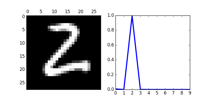
>>> print("Image number {0} is a {1}, and the network predicted a {2}".format(imgnr, test_data[imgnr][1], np.argmax(prediction)))
Image number 4709 is a 2, and the network predicted a 2
>>> import matplotlib.pyplot as plt
>>> fig, ax = plt.subplots(1,2,figsize=(8,4))
>>> ax[0].matshow( np.reshape(test_data[imgnr][0], (28,28) ), cmap='gray' )
>>> ax[1].plot( prediction, lw=3 )
>>> ax[1].set_aspect(9)
>>> plt.show()
	

⊕ A convolutional network is another way to link neurons. The layers in such a network are not fully-connected. Here is an example convolutional neural network for the MNIST Data Set. It reaches a 98.80% accuracy. The trained network predicts that the image (chosen randomly) is a "2."