Philosophy, Computing, and Artificial Intelligence
PHI 319. Technical Background and Foundations of Logic Programming.
 Computational Logic and Human Thinking
A1-A3 (251-283), A5 (290-300)
Thinking as Computation
Chapter 2 (23-39)
Logic and Logic Programming
This lecture looks much more difficult than it is.
Be patient!
The ideas are
beautiful, but they take some
effort to see.
Don't worry if you don't understand every detail.
To do well in the
course, you only need to understand enough to write thoughtful discussion posts and
to answer the questions in the
assignments.
Remember too that you can post questions about anything in the lectures or in the assignments.
Posting questions is a good way to learn because just formulating a question helps
makes the issues clearer.
Logic programming was developed to construct a better computer language.
The first computer languages took their form from early attempts to solve what, in 1928, David Hilbert and Wilhelm Ackermann called the Entscheidungsproblem" (and translates into English as "decision problem"). They wanted to know whether there are easy to follow instructions to determine the answer ("yes" or "no") to any mathematical question.
To solve the Entscheidungsproblem, it is necessary to understand what counts as "a set of easy to follow instructions." In 1936, Alan Turing provided an answer. He gave a theoretical description of a machine with the ability to execute instructions. It was thought that a set of instructions counted as easy to follow if they were instructions the machine could execute.
The attempt to build such machines became part of the effort to win the Second World War. In 1942, John Mauchly and Presper Eckert set out the technical outline of a machine to compute the trajectories of artillery shells. This machine, ENIAC (Electronic Numerical Integrator and Computer), was built in 1946. To carry out a new set of instructions, ENIAC had to be rewired manually. To overcome this problem, Mauchly and Eckert turned worked to design EDVAC (Electronic Discrete Variable Automatic Computer). In this same period, John von Neuman had been working on the Manhattan Project to develop nuclear weapons. He recognized that the new computing machines could help carry out the necessary calculations to understand and build these weapons. He joined Mauchly and Eckert, and he produced a technical report describing EDVAC. A machine with this design was built in 1949.
The conceptual model in the design in the technical report for EDVAC became known as the von Neuman architecture. Computers built according to this architecture were called von Neuman machines. The instructions a von Neuman machine executes were easy to follow. They were of the sort "place the sum of the contents of addresses a and b into address c."
It is true that instructions of this sort are easy to follow, but thinking about how to create lists of such instructions to solve problems is not natural for most people. This led to an attempt to design languages that abstracted away from the architecture of the machine. The goal in this abstraction was to make the language more natural for human beings to understand. Many languages developed in early computer science (such as the C programming language) did not go very far. They remained heavily influenced by the architecture of the machine.
The language of logic programming is completely different in this respect.
The Language of Logic Programming
The language of logic programming is roughly the language of the first-order predicate calculus. This language come out of the work of the philosopher Gottlob Frege (1848-1925). He developed it to clarify certain issues in mathematics and its relation to logic.
A logic program can be understood as a formula of the first-order predicate calculus (FOL).
The logic program from the first lecture provides a straightforward example:
a ← b, c.
a ← f.
b.
b ← g.
c.
d.
e.
We can think of this program as a set of beliefs (or KB). These beliefs, so understood, are symbolic structures we can represent as formulas in the language of FOL.
∨ symbolizes disjunction: "b or c." The letters
b and c stand for declarative sentences. (In Latin, the word
for "or" is
vel.)
A disjunction has disjuncts. In the disjunction a ∨ ¬b ∨ ¬c,
the disjuncts are a, ¬b, and ¬c.
∧ symbolizes conjunction: "b and c." The letters b
and c stand for declarative sentences. Whereas a disjunction has disjuncts, a conjunction has conjuncts. In
the conjunction b ∧ c, the conjuncts are b and c.
The English word 'atomic' derives from the Greek adjective
ἄτομος.
One of the meanings of this adjective is "uncuttable" and thus "without parts."
An atomic formula is a formula not composed of other formulas.
¬ symbolizes negation: "It is not the case that b." The letter
b stands for a declarative sentence.
To talk about this, it helps to fix the meaning of some terms.
• A clause is a disjunction of literals.
a ∨ ¬b ∨ ¬c is a clause. a ← b, c is another way to write this clause.
• A literal is an atomic formula or the negation of an atomic formula.
a is an atomic formula.
¬b, ¬c are negations of atomic formulas.
• A positive literal is an atomic formula.
a is a positive literal. Positive literals symbolize declarative sentences.
• A negative literal is the negation of an atomic formula.
¬b, ¬c are negative literals. Negative literals symbolize the negations of declarative sentences.
• A definite clause contains exactly one positive literal
and zero or more negative literals.
a ∨ ¬b ∨ ¬c is a definite clause.
• A definite logic program is a conjunction (or set) of definite clauses
Here are some more definitions:
• A negative clause contains zero or more negative literals
and no positive literals.
• The empty clause is a
negative clause with zero negative literals. To signify the empty clause, we use the symbol ⊥.
• A Horn clause is a definite clause or a negative clause.
(These clauses are named for mathematician
Alfred Horn.)
• Negative clauses are queries or goal clauses.
• An indefinite clause contains at least two positive
literals and zero or more negative literals. An indefinite logic
program is a conjunction (or set) of clauses that contains at least
one indefinite clause. A logic program is a definite logic
program or an indefinite logic program.
The example logic program is a
definite logic program. Definite logic programs are the kinds of logic programs we will use
in our attempt to model the intelligence of a rational agent.
The Propositional Calculus
What is sometimes called the propositional calculus is a simplified form of the first-order predicate calculus. In philosophy classes in symbolic logic, it is traditional to think about the propositional calculus as an introduction to the first-order predicate calculus.
We can represent sentences in English as formulas in the propositional calculus.
These formulas are composed of atomic formulas
and truth-functional connectives (¬, ∧, ∨, →). The
atomic formulas have no parts (hence their name) and are the formulas from which
we construct compound formulas of the language.
In philosophy, it is common to say that declarative sentences
express propositions. This terminology explains why the calculus constructed from atomic
formulas and truth-functional connectives is called the
propositional calculus.
In philosophy, it is traditional to use capital letters from the end
of the alphabet (P, Q, R, ...) for atomic
formulas. In logic programming, it is traditional to use small letters from
the beginning of the alphabet (a, b, c, ...).
We construct the compound formulas from formulas with fewer connectives:
φ and ψ are metalinguistic variables. Metalinguistic variables have strings
of the language are their values.
¬φ is shorthand for ⌜¬φ⌝. ⌜¬φ⌝ denotes the concatenation of the string ¬ with
the string that is the value of φ.
If, for example, the value of
φ is (P ∧ Q),
then the value of
⌜¬φ⌝ is ¬(P ∧ Q).
if φ is a formula, then ¬φ is a formula
¬φ is the negation of φ. Read ¬φ as "not φ"
¬b and ¬c are examples
if φ and ψ are formulas, then (φ ∧ ψ) is a formula
(φ ∧ ψ) is the conjunction of φ and ψ. Read (φ ∧ ψ) as "φ and ψ"
b ∧ c is an example
if φ and ψ are formulas, then (φ ∨ ψ) is a formula
(φ ∨ ψ) is the disjunction of φ and ψ. Read (φ ∨ ψ) as "φ or ψ"
¬b ∨ ¬c is an example
if φ and ψ are formulas, then (φ → ψ) is a formula
(φ → ψ) is the implication of ψ from φ. Read (φ → ψ) as "if φ, then ψ"
(b ∧ c) → a is an example
Parentheses eliminate ambiguity. We drop outside parentheses to increase readability.
The Example Logic Program
"The central component of a knowledge-based agent is its knowledge
base, or KB. A knowledge base is a set of sentences. (Here
'sentence' is used as a technical term. It is related but not identical to the
sentences of English and other natural languages.) Each sentence is expressed
in a language called a knowledge representation language and represents
some assertion about the world. ... There must be a way to add new sentences
to the knowledge base and a way to query what is known. The standard names for
these operations are TELL and ASK, respectively. Both operations may involve
inference —that is, deriving new sentences from old. Inference must obey the
requirement that when one ASKs a question of the knowledge base, the answer
should follow from what has been told (or TELLed) to the knowledge base
previously" (Russell & Norvig,
Artificial Intelligence. A Modern Approach, 235).
Russell and Norvig tell us that "[i]nference must obey the
requirement that ... the answer
should follow from...."
Why?
What does "follow from" mean?
Now that we have a grasp of the languages of logic programming and the propositional calculus, we can begin to see how we can understand logic programs as formulas in FOL.
Here, again, is the example logic program from the first lecture:
a ← b, c.
a ← f.
b.
b ← g.
c.
d.
e.
Consider the first line in this program.
a ← b, c.
It is what in logic programming is called a "rule." (The second and fourth entry are also rules.) We can understand this rule as a way to write the backward-arrow conditional
a ← b ∧ c
This backward-arrow conditional is itself a way to write
(b ∧ c) → a
It is enough for now to understand truth-functionally equivalent
to mean that the formulas saying the same thing because
they evaluate to the same truth-value.
Here is a trivial example: a ∧ b and b ∧ a. These formulas are
trivially different ways to say the same thing.
This formula, in turn, is truth-functionally equivalent to
a ∨ ¬(b ∧ c)
The second disjunct in this formula
¬(b ∧ c)
is truth-functionally equivalent to
¬b ∨ ¬c
So we can understand each line in logic program as a formula in the propositional calculus:
a ∨ ¬b ∨ ¬c
a ∨ ¬f
b
b ∨ ¬g
c
d
e
If we think of this logic program as a "knowledge base" (KB), then we have made some progress in our attempt to model of the intelligence of a rational agent. We have a model of the beliefs in terms of which a rational agent thinks about the world and decides what to do.
Truth and Falsehood
"[An] issue to consider is grounding—the connection between logical reasoning
processes and the real environment in which the agent exists. In particular, how do we know
that KB is true in the real world? (After all, KB is just 'syntax' inside the agent’s head.)
This is a philosophical question about which many, many books have been written. ...
A simple answer is that the agent’s sensors create the connection. For example,
our wumpus-world agent has a smell sensor. The agent program creates a suitable sentence
whenever there is a smell. Then, whenever that sentence is in the knowledge base, it is
true in the real world. Thus, the meaning and truth of percept sentences are defined by the
processes of sensing and sentence construction that produce them"
(Artificial Intelligence. A Modern Approach, 243)
This "simple answer" is not very helpful. Perception, as it is usually understood, is not veridical. In the "simple answer," there is
a lot going on behind the curtain when "[t]he agent creates
a suitable sentence whenever there is a smell."
"Falsehood and error always depend upon the intrusion of opinion"
(Epicurus, Letter to Herodotus,
X.50).
What an agent believes can be true or false.
For an agent whose beliefs we are using the example logic program to model, we need a key to assign meanings to the structures in the KB. The initial part of this key might be
a = "I can open the door"
b = "I can twist the knob"
c = "I can pull the door"
Given this key, is the proposition that "a ← b, c" represents true?
This proposition seems true, but we can easily imagine that in other cases it may be hard to know with any certainty whether the propositions in a KB are true or false.
The agent must solve this problem. Its beliefs must be sensitive to evidence.
This presents an enormous challenge for our attempt to model the intelligence of a rational agent, but for now we set it aside and use a technical device to help us understand an important logical property of the method we use in logic programming to compute answers to queries.
The technical device is truth or falsehood in a model. To construct this device, we define an interpretation function to assign truth-values (true or false) to the formulas.
Each interpretation function has two parts. The first part of the function is from the atomic formulas to true (T) or false (F). The second part extends the first to all the formulas in a way that respects the truth-functional meanings of the connective symbols (¬, ∧, ∨, →).
Each row in the following table displays a part of an interpretation function:
   φ         ψ       ¬φ       φ ∧ ψ      φ ∨ ψ      φ → ψ
   T         T         F             T              T             T
   T         F         F              F              T             F
   F         T         T             F              T             T
   F         F         T              F              F             T
Given truth-values for φ and ψ, each interpretation function assigns compound formulas truth-values according to the truth-functions for the connectives (¬, ∧, ∨, →).
For the example logic program, the first part of one possible interpretation function, I, is
I(a) = false
I(b) = true
I(c) = true
Relative to this interpretation function, the formula a ← b, c is false.
We can easily check this.
As we have seen, the formula a ← b, c in the logic program reduces to
a ∨ ¬b ∨ ¬c
If we replace the literals with their truth-values, we get
false ∨ ¬true ∨ ¬true
If we look at how the interpretation function behaves for the connectives ∨ and ¬, it is clear that each disjunct in a ∨ ¬b ∨ ¬c is false and hence that the disjunction is false.
Keep in that true and false and true and false in a model need not coincide. We define interpretation functions so that they assign true and false to the atomic formulas arbitrarily.Given the notion of truth in a model, we are now ready to see an important logical property of the method of computing (we are calling backward chaining) logic programming uses.
Models and Backward Chaining
Another reason to take an interest in models (which will be familiar to many who have taken an introductory class in symbolic logic) is that they characterize certain classes of formulas. So, for example, if every interpretation is a model of a given formula, then the formula is a tautology. An interpretation function is a model of a set of formulas just in case the function makes all the formulas true. In the context of logic programming, we are interested in these interpretation functions we call models because we want to know whether backward chaining is sound.
To understand what it is for backward chaining to be sound, consider first the example logic program (on the left side of the hashed vertical line) and its corresponding formulas:
a ← b, c.      |       a ∨ ¬b  ∨ ¬c
a ← f.          |       a ∨ ¬f
b.                |       b
b ← g.         |       b ∨ ¬g
c.                |       c
d.                |       d
e.                |       e
To specify a model, we need to specify an interpretation function that makes all the formulas true. Here is a possible interpretation function, I, for the atomic formulas:
I(a) = true
I(b) = true
I(c) = true
I(d) = true
I(e) = true
I(f) = false
I(g) = false
Given this assignment of true and false to the atomic formulas, the extension of this interpretation function to compound formulas makes all the clauses in the logic program true.
We can easily check this.
Consider the first line, a ← b, c. In the propositional calculus, the formula that corresponds to a ← b, c is a ∨ ¬b ∨ ¬c. This is a disjunction, and a disjunction is true just in case at least one disjunct is true. So, since I assigns true to a, it assigns true to a ∨ ¬b ∨ ¬c.
Backward Chaining is Sound
⊥ is the empty clause. It is a disjunction with no disjuncts.
⊥ is false. Why? A disjunction is true just in case a least one of disjuncts is
true. ⊥ has no disjuncts, so none are true.
KB U {¬a} ⊢ ⊥ says that ⊥ is a logical
consequence of KB and ¬a. This means there is a
logical deduction of ⊥ from premises in the set consisting of
¬a and the formulas in KB.
Backward chaining gives a positive answer for query a relative to a KB only if
KB U {¬a} ⊢ ⊥.
If KB U {¬a} ⊢ ⊥, then KB ⊢ a.
If KB ⊢ a, then KB ⊨ a.
KB ⊨ a says that KB logically entails a.
This means that a is true in every model that makes all the formulas in
KB true.
Suppose that the beliefs in the KB are true and that backward chaining gives a positive answer to a query.
Can we conclude, in these circumstances, that the query true?
The answer is "yes" if backward chaining is sound. If backward chaining is sound, (and it is although we will not prove it), the query is true in every model of the beliefs in the KB.
Consider the following very simple logic program
a ← b.
b.
This program can be understood as the formulas
a ∨ ¬b
b
Now suppose the query is
?-a.
To answer this query, we start the backward chaining computation. We begin with a top down search to determine whether the query (a) matches the head of an entry in the KB. It does. It matches the head of the first entry (a ← b). Given a match, we push the tail of the entry (b) onto the query list. So the list is now b. Because we process this list last in first out, we pass b as a query to the KB. It matches the the head of the second entry (b). Facts have no tail, so there is nothing to push onto the query list. This means that the query list is empty, and this causes the backward chaining procedure to stop and the query to be answered positively.
Is a true on every interpretation that makes the beliefs in the KB true?
Yes.
Why?
It is impossible to assign truth-values so that a is false and a ∨ ¬b and b are true.
Why?
Because if b is true, then ¬b is false and thus a ∨ ¬b is false if a is false.
Backward Chaining Searches for a Proof
The backward chaining computation is sound because it searches for a proof that the query is a logical consequence of the KB. The algorithm does not always find the shortest or most elegant proof. It implements a search for what is called a reductio ad absurdum proof.
"Sentences are physical configurations of the agent, and reasoning is a process
of constructing new physical configurations from old ones. Logical reasoning should ensure
that the new configurations represent aspects of the world that actually follow from the
aspects that the old configurations represent"
(Russell & Norvig,
Artificial Intelligence. A Modern Approach, 243).
What does "actually follow from" mean here?
This understanding of what the backward chaining computation does can be more than a little
surprising. Initially the computation does not look like a search for a
proof. It looks like a series of mindless steps in an
algorithm: matching heads, pushing derived queries onto the query list, and so on.
If, however, we think abstractly about these steps, we can see that they implement a certain form of
intelligence. In our model of a rational agent, they implement the ability to engage in logical deduction (the
process of deducing logical consequences).
It seems plausible to think a similar relationship holds between processes involving neurons in the human brain and the forms of intelligence that belong to human beings. We recognize the ability to engage in logical deduction as a form of intelligence, and it seems that somehow or another biochemical processes involving neurons implement the exercise of this ability.
The Proof in the Very Simple Example
In what follows, I give the proof (in a
Gentzen-style natural deduction) that
backward chaining finds for the query in the case of the very simple logic
program.
Gerhard Gentzen
(1909-1945) was a mathematician and logician who did the pioneering work in
proof theory.
It is not necessary in this course to understand the proof (which looks much harder to understand than it is). I give it for those who are interested.
There is a shorter proof, but it is not a reductio ad absurdum:
[¬b]2 b
-------
⊥
-----
a ∨ ¬b [a]1 a
---------------------
a
Here is this shorter proof in the Fitch style:
(In logic classes
in philosophy, it is traditional to use P, Q, R, and so on, for atomic formulas)
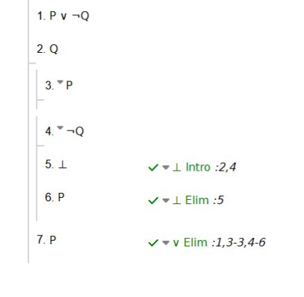 In this proof, red marks the rule (a ∨ ¬b)
and the fact (b). Blue marks the negative
clause (¬a) corresponding to the query.
This negative clause is the assumption for reductio in the proof.
In this proof, red marks the rule (a ∨ ¬b)
and the fact (b). Blue marks the negative
clause (¬a) corresponding to the query.
This negative clause is the assumption for reductio in the proof.
                             [a] 1    [¬a]3
                             -----------  ¬E
                                    ⊥
                                 ------ ⊥I
     a ∨ ¬b                  ¬b                          [¬b]2
    -----------------------------------------  ∨E, 2, 3
                                                    ¬b                                          b
                                                    ----------------------------- ¬E
                                                                            ⊥
                                                                          ----- ¬I, 1
                                                                          ¬¬a
                                                                         ------ ¬¬E
                                                                             a
To show how this proof works, it is helpful to divide it into three parts.
The first of these parts shows that from the premises a ∨ ¬b (which corresponds to the first entry in the logic program) and ¬a (which is the negative clause that corresponds to the query), the conclusion ¬b is a logical consequence:
                  [¬a]3
                 ---------------
                            .
                            .
                            .
  a ∨ ¬b
  ---------------------------------------
                                  ¬b
The second part of the three parts of the proof extends the first. It shows that given the first part of the proof and given b (which is the fact in the KB), it follows that ⊥:
                  [¬a]3
                 ---------------
                            .
                            .
                            .
  a ∨ ¬b
  ---------------------------------------
                                  ¬b                                               b
                                 --------------------------------
                                                           ⊥
The pattern here corresponds to the matching procedure in backward chaining. The negative clause ¬a (the logical form of the query a) together with a ∨ ¬b (the logical form of the rule) are premises in a proof of the negative clause ¬b (the logical form of the derived query b):
                                             ¬a       a ← b  (or: a ∨ ¬b)
                                              |          /
                                              |       /
                                              |     /
                                              |   /
                                              ¬b     b
                                              |       /
                                              |    /
                                              |  /
                                               ⊥
If the derived query is is ⊥, the derived query list is empty. The backward chaining process stops when there are no more derived queries and returns a positive answer to the initial query a. This success is specified in the final part of the proof by the derivation of a from ¬¬a.
The Logic Programming/Agent Model
We use the backward chaining computation to model a form of intelligence.
This intelligence is the ability to answer the question "is this proposition a logical consequence of what I believe and thus true in every model that makes my beliefs true."
This is not the ability to answer the question "should I believe this proposition."
To see the difference more clearly, consider how human beings form beliefs on the basis of perception. It can be rational to believe that a given object is red if it looks red. We form beliefs this way all the time, but being red is not a logical consequence of looking red.
It would be great if we could model this second ability we see in human intelligence, but for now we settle for what we can compute. We settle for computing logical consequence.
"Logical AI has both epistemological problems and heuristic problems. The former concern the knowledge needed by an intelligent agent and how it is represented. The latter concerns how the knowledge is to be used to decide questions, to solve problems and to achieve goals. ... Neither the epistemological problems nor the heuristic problems of logical AI have been solved" (John McCarthy, "Concepts of Logical AI," 2000).
Why do we settle for this?
Logical consequence, first of all, is something we can compute.
This achievement is an important step forward in the history of AI.
Logical consequence, moreover, is useful. If a rational agent believes P and discovers that Q is a logical consequence of P, then the agent has increased its knowledge about itself and the world.
The ability to compute logical consequences is thus a first step in our project of using techniques from logic to construct a model of the intelligence of a rational agent.
The First-Order Predicate Calculus
Now we turn to the more general language of the first-order predicate calculus.
The first-order predicate calculus is more expressive than the propositional calculus. It allows for the representation of some propositions the propositional calculus does not represent well.
Consider, for example, the following simple argument
1. Bachelors are not married
2. Tom is a bachelor
----
3. Tom is not married
This argument is valid, but its validity is not captured when the argument is represented in the propositional calculus. In the propositional calculus, the argument is something like
1. P
2. Q
----
3. R
This representation leaves out too much detail to capture the validity of the argument. We need to expose the name (Tom) and the two predicates (is a bachelor, is married).
The first-order predicate calculus provides a way to do this.
Syntax for the First-Order Predicate Calculus
The vocabulary of the first-order predicate calculus subdivides into two parts, a logical and a nonlogical part. The logical part is common to all first-order theories. It does not change. The nonlogical part varies from theory to theory. The logical part of the vocabulary consists in
• the connectives: ¬ ∧ ∨ → ∀ (universal quantifier) ∃ (existential quantifier)
• the comma and the left and right parenthesis: , ( )
• a denumerable list of variables: x1 x2
x3 x4. . .
The nonlogical part of the vocabulary consists in
• a denumerable list of constants: a1 a2
a3 a4. . .
• for each n, a denumerable list of n-place
predicates:
P1
1,
P1
2,
P1
3, . . .
P2
1,
P2
2,
P2
3, . . .
P3
1,
P3
2, . . .
and so on for each n
Given the vocabulary, a formula is defined as follows:
• If Pn is a n-place predicate, and
t1, ..., tn are terms,
A term is
either a variable or a constant.
Pnt1, ..., tn is a
formula
• If φ and ψ are formulas, ¬φ, (φ ∧ ψ), (φ ∨ ψ), (φ
→ ψ) are
formulas
• If φ is a formula and v is a
variable, then ∀vφ, ∃vφ are formulas
• Nothing else is a formula
This looks more complicated than it is. All we are really doing in setting out the syntax is saying how to construct formulas from the basic pieces in the language.
Semantics for the First-Order Predicate Calculus
"The language of first-order logic ... is built around objects and relations. It has been so important to mathematics, philosophy, and artificial intelligence precisely because those fields—and indeed, much of everyday human existence—can be usefully thought of as dealing with objects and the relations among them. First-order logic can also express facts about some or all of the objects in the universe. ... The primary difference between propositional and first-order logic lies in the ontological commitment made by each language—that is, what it assumes about the nature of reality. Mathematically, this commitment is expressed through the nature of the formal models with respect to which the truth of sentences is defined. For example, propositional logic assumes that there are facts [or: propositions] that either hold or do not hold in the world. Each fact can be in one of two states: true or false, and each model assigns true or false to each proposition symbol.... First-order logic assumes more; namely, that the world consists of [a domain of] objects with certain relations among them that do or do not hold" (Russell & Norvig, Artificial Intelligence. A Modern Approach, 289). Models of formulas in FOL are representations of things in the world and their relations to each other. These models are different from the models for the propositional calculus, but their function is the same: they allow for the statement of truth-conditions.
• A model is an ordered pair <D,
F>, where D is a domain and
F is an interpretation. The domain D is a non-empty set that
contains things the formulas are about. The interpretation, F, is a function on the
non-logical vocabulary. It gives the meaning of this vocabulary relative to the domain.
For every constant c, F(c) is in D. F(c) is the referent
of c in the model.
For every n-place predicate Pn,
F(Pn) is a subset of
Dn. F(Pn) is the
extension of Pn in the model.
• An assignment is a function from variables to members
of D. A v-variant of an assignment
g is an assignment that agrees with g except
possibly on v.
The truth of a formula relative to a model and an assignment is defined inductively. The base case uses the composite function [ ] F g on terms, defined as follows:
[t] F g = F(t) if t is a constant. Otherwise, [t] F g = g(t) if t is a variable.
The clauses in the inductive definition of truth relative to M and g are as follows:
Pnt1,...,
tn is true relative to M and g iff
<[t]
F g, ...,
[t]
F g> is in
F(Pn).
¬A is true relative to M and g if A
is not true relative to M and g.
A ∧ B is true relative to M and g if
A and B are true relative to M and g.
A ∨ B is true relative to M and g if
A or B is true relative to M and g.
A → B is true relative to M and g if
A is not true or B is true relative to M and g.
∃vA is true relative to M and g if A
is true relative to M and g*, for some v-variant
g* of g.
∀vA is true relative to M and g if A
is true relative to M and g*, for every v-variant
g* of g.
A formula is true relative to a model M iff it is true relative to M for every assignment g.
Again, this all looks much more complicated than it is. In setting out the semantics, we are just saying how to determine whether a formula is true in a given model.
An Example in Prolog Notation
A statement of the syntax and semantics of the first-order predicate calculus is necessary for understanding logical properties like soundness, but it is not very user friendly.
We need a a more intuitive language, and Prolog is such a language.
In Prolog, a variable starts with an upper-case letter and a constant starts with a lower-case letter.
This example is from Representation and Inference for Natural Language: A First Course in Computational Semantics. We can use this syntax to set out a simple KB based on the now old but once popular movie Pulp Fiction. In this movie, various people both love other people and are jealous of other people. To simplify what is true in the movie, we will suppose that a certain rule defines jealousy. So, in the language of Prolog, the KB that represents common knowledge is
loves (vincent, mia).
"Vincent loves Mia."
loves (marcellus, mia).
"Marcellus loves Mia."
loves (pumpkin, honey_bunny).
"Pumpkin loves Honey Bunny."
loves (honey_bunny, pumpkin).
"Honey Bunny loves Pumpkin."
jealous (X, Y) :- loves (X, Z), loves (Y, Z).
This rule for jealousy is interpreted as a universal quantified formula:
This is not a formula of Prolog or the first-order predicate calculus. It is a mixed form, meant to be suggestive. ∀X ∀Y ∀Z ( ( loves (X, Z) ∧ loves (Y, Z) ) → jealous (X, Y) )
The symbols X, Y, and Z are variables. The rule is universal. It says that x is jealous of y if x loves z and y loves z. Obviously, jealousy in the rule and the real world are different.
To represent this KB in the language of FOL, we need to map the constants and predicates in Prolog to constants and predicates in FOL. Here is one possibility:
Vincent a1
Marcellus a2
Mia a3
Pumpkin a4
Honey Bunny a5
__ loves __ P2
1
__ is jealous of __ P2
2
Now it is possible to interpret the entries in the KB as FOL formulas.
loves (marcellus, mia), for example, would map to P2 1a2,a3. The language of the first-order predicate calculus is traditionally set out in this unfriendly way to make it easy to prove various things about the language.
Prolog notation thus can be translated into FOL, but the Prolog notation is easier to read.
To set out a model <D, F> for the "Pulp Fiction" KB, we need to define the domain D and the interpretation F. The domain is straightforward. It consists in the people in the movie
D = {Vincent, Marcellus, Mia, Pumpkin, Honey Bunny}.
The interpretation F in the model <D, F> is a little more complicated to set out. It assigns the constants to members of the domain D. So, for example,
F (a1) = Vincent
The interpretation F also assigns extensions to the predicates. For F (P21), it is the set of pairs from the domain such that the first in the pair loves the second in the pair
F (P21) =
{<Vincent, Mia>,
<Marcellus, Mia>,
<Pumpkin, Honey Bunny>,
<Honey Bunny, Pumpkin>}
In this model <D, F>, the formula P2 1a2,a3 is true.
Queries to the "Pulp Fiction" Program
Relative to the example KB taken from the Movie Pulp Fiction,
loves (vincent, mia).
loves (marcellus, mia).
loves (pumpkin, honey_bunny).
loves (honey_bunny, pumpkin).
jealous (X, Y) :- loves (X, Z), loves (Y, Z).
consider the following query (whether Mia loves Vincent):
?- loves (mia, vincent).
The response is
false (or no, depending on the particular implementation of Prolog)
For a slightly less trivial query, consider
?- jealous (marcellus, W).
This asks whether Marcellus is jealous of anyone. In the language corresponding to the first-order predicate calculus, the query asks whether there is a w such that Marcellus is jealous of w:
∃W jealous (marcellus, W)
Since Marcellus is jealous of Vincent (given the KB), the response is
W = vincent
From a logical point of view, the query (and the answer to the query is computed in terms of) the corresponding negative clause
¬jealous(marcellus, W)
This negative clause is read as its universal closure
∀W ¬jealous(marcellus, W)
which (by the equivalence of ∀ to ¬∃¬ in classical logic) is equivalent to
¬∃W jealous(marcellus, W)
The computation (to answer the query) corresponds to the attempt to refute the universal closure by trying to derive the empty clause. Given the KB, the empty clause is derivable
{KB, ∀W ¬jealous(marcellus,W)} ⊢ ⊥
This means (given the equivalence of ∀ to ¬∃¬ and of ¬¬φ and φ in classical logic) that
∃W jealous (marcellus,W)
is a consequence of the KB. Moreover, the computation results in a witness to this existential formula. Given the KB, Marcellus is jealous of Vincent. So the response to the query is
W = vincent
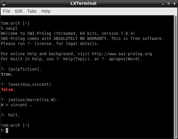
Here is how this "thinking" looks when it is implemented on my laptop with SWI-Prolog:
A Corresponding Proof in the Predicate Calculus
As in the case of the propositional logic, a backward chaining computation that issues in a positive response to a query corresponds to a reductio ad absurdum proof in FOL.
I set out this proof as a Gentzen-style natural deduction. Red marks two facts and the rule. Blue marks the negative clause corresponding to the query. This is the assumption for reductio.
To make the proof fit nicely on the page, I abbreviate the predicates "loves" and "jealous" as "l" and "j" and abbreviate the constants "marcellous" and "vincent" as "mar" and "vinc."
Note also that ¬∀x¬ ("not all not") is equivalent to ∃ ("some") in classical first-order logic.
                                                     ∀x∀y∀z((l(x,z) ∧ l(y,z)) → j(x,y))
                                                     ---------------------------------- ∀E
                                                     ∀y∀z((l(mar,z) ∧ l(y,z)) → j(mar,y))
                                                     ----------------------------------- ∀E
l(mar,mia)     l(vinc,mia)            ∀z((l(mar,z) ∧ l(vinc,z)) → j(mar,vinc))
---------------------- ∧I     ------------------------------------- ∀E
 l(mar,mia) ∧ l(vinc,mia)         (l(mar,mia) ∧ l(vinc,mia)) → j(mar,vinc)          [∀x¬j(mar,x)]1
------------------------------------------------------------------ →E     --------------- ∀E
                                                                  j(mar,vinc)                                             ¬j(mar,vinc)
                                                                 --------------------------------------------------- ¬E
                                                                                                                  ⊥
                                                                                                                ----- ¬ I, 1
                                                                                                                ¬∀x¬j(mar,x)
Unification is Part of the Computation
The instantiation of variables is a complicating factor. Now (unlike for the propositional calculus) the backward chaining computation includes what is called unification.
Notice that in the "Pulp Fiction" example, the query
jealous (marcellus, W)
matches the head of no entry in the logic program, but it can be "unified" with the head of the rule for jealousy. Unification, in this way, is a substitution that makes two terms the same.
A substitution is a replacement of variables by terms. A substitution σ has the following form
{V1/t1, ... , Vn/tn}, where VI is a variable and ti is a term.
φσ is a substitution instance of φ. It is the formula that results from the replacement of every free occurrence of the variable Vi in φ with the term ti.
An example makes unification a lot easier to understand.
Consider the following
blocks-world logic program:
on(b1,b2).
on(b3,b4).
on(b4,b5).
on(b5,b6).
above(X,Y) :- on(X,Y).
above(X,Y) :- on(X,Z), above(Z,Y).
If we use our imagination a little, we can see that an agent with this logic program as its KB thinks that the world consists in an arrangement of blocks that looks like this:
          b3
          b4
 b1     b5
 b2     b6
Now suppose the query is whether block b3 is on top of block b5
?- above(b3, b5).
The backward chaining computation to answer (or solve) this query runs roughly as follows. The query does not match the head of any fact. Nor does it match the head of any rule. It is clear, though, that there is a substitution that unifies it and the head of the first rule.
The unifying substitution is
{X/b3, Y/b5}
This substitution produces
above(b3,b5) :- on(b3,b5).
So the derived query is
on(b3,b5).
This derived query fails. So now it is necessary to backtrack to see if another match is possible further down in the knowledge base. Another match is possible. The query can be made to match the head of the second rule. The unifying substitution is
{X/b3, Y/b5}
This produces
above(b3,b5) :- on(b3,Z), above(Z,b5).
The derived query is
on(b3,Z), above(Z,b5).
Now the question is whether the first conjunct in this query can be unified with anything in the KB. It can. The unifying substitution for the first conjunct in the derived query is
{Z/b4}
The substitution has to be made throughout the derived query. So, given that the first conjunct has been made to match, the derived query becomes
above(b4,b5).
This can be made to match the head of the first rule. The unifying substitution is
{X/b4, Y/b5}
and the derived query is now
on(b4,b5}.
This query matches one of the facts in the knowledge base. So now the query list is empty and hence the computation is a success! The query is a logical consequence of the KB.
We can set out the computation (together with the substitutions) in the following form:
    ¬above(b3,b5)     above(X,Y) :- on(X,Z), above(Z,Y)                   {X/b3, Y/b5}
                                 above(X,Y) ∨ ¬on(X,Z) ∨ ¬above(Z,Y)
        \
         \                   /
          \                 /
    ¬on(b3,Z) ∨ ¬above(Z,b5))         on(b3,b4)                                    {Z/b4}
                     \                                      /
                      \                                   /
                       \                              /
                            ¬above(b4,b5)            above(X,Y) :- on(X,Y)           {X/b4, Y/b5}
                                                                above(X,Y) ∨ ¬on(X,Y)
                                     \                       /
                                      \                    /
                                         ¬on(b4,b5)         on(b4,b5)
                                              \                 /
                                               \              /
                                                      ⊥
What we have Accomplished in this Lecture
We examined the relation between logic and logic programming. We saw that if a query to a logic program (or KB) is successful (results in a positive response), then the query is a logical consequence of premises taken from the logic program. To see this, we considered the connection between the backward chaining process in computing a successful query and the underlying proof in the propositional and first-order predicate calculus.
We saw that backward chaining in logic programming implements a form of intelligence: the ability to deduce logical consequences. We saw examples of backward chaining working on a machine and thus saw that a machine can implement a form of intelligence.
We saw that in human intelligence there is the ability to answer the question should I believe this proposition. We saw that the logic programming/agent model, in its current form, does not have this form of intelligence. It, instead, has the ability to compute some logical consequences of the the KB, and rational agents have a lot more intelligence than this.